Editorial
Mustache to Touch – Visualizing Model Risk for Exotics
For vanilla options, the volatility smile shows the implied volatility in the Black-Scholes model and is interpreted as the deviation of the market from the normal returns assumed by the Black-Scholes model. Since the relationship of volatilities and vanilla option prices is monotone, this way to visualize the market- or model-implied deviation is the established standard.
We visualize the USD/JPY volatility smile of the market data of 23 January 2018 in Figure 1. Spot reference was 110.31 and out-of-the-money puts are higher priced than out-of-the-money calls.
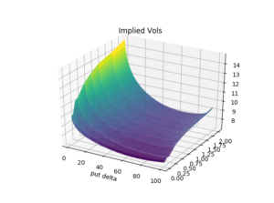
Figure 1: USD/JPY volatility surface of 23 Jan 2018, put forward delta on the x-axis, time to maturity on the y-axis, implied volatility on the z-axis – raw data sourced from Bloomberg, surface built by MathFinance.
Therefore, for pricing vanilla options, it is common to use the Black-Scholes formula, and all the quantitative/modeling work is shifted to and hidden in the way the volatilities are interpolated and extrapolated on both the strike-space and maturity space (Smile). It is only for pricing exotics that we really need a model. The common industry models include vanna-volga (Vv2), local volatility (Lv), stochastic volatility (Sv100) and stochastic-local-volatility mixture models with a mixing factor of 75% (Slv75), where 75 is just an example.
We visualize in Figure 2 how the models can be calibrated to the vanilla options market: Obviously, Smile, Lv and Slv75 fit the vanilla option prices by construction and exhibit a flat line. Vv2 and Sv100 don’t fit the vanilla smile perfectly, particularly not on the wings. Vv2 does not take the information beyond 25-delta into account, thus a good fit for low deltas or far away strikes is not expected. Sv100 does to the best possible fit via minimization of the distance of the model from the market. Consequently, even this stochastic volatility approach is not expected to yield a perfect fit.
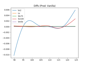
Figure 2: USD/JPY model fit of 23 Jan 2018, strike on the x-axis, and differences to ATM volatility on the y-axis, raw data sourced from Bloomberg, calculations by MathFinance.
This was the reason why 100% stochastic volatility models, like Heston, needed a local-volatility model mix, to fit the market input consistently. Local volatility models alone can fit the vanilla option prices for one maturity perfectly, but tend to misprice path-dependent claims, e.g. tend to overprice touch contracts. Therefore, one either starts with a stochastic volatility model, adds a local volatility to straighten up calibration to fit the vanilla option prices, or one starts with local volatility models and mixes them randomly, the so-called local-volatility mixture approach.
We illustrate the effect for a 9-month one-touch contract in USD/JPY with a touch-level below initial spot. A common way to visualize the model-impact is to use the x-axis for the theoretical value (TV) of the One-Touch, and the difference to the TV on the y-axis for the other models. Note that the touch level is varied to create TVs ranging from 0=0% (touch level very far from spot) and 1=100% (touch level on the spot). As a result, the Slv75 comes to lie between the Sv100 and the Lv, as can be see in Figure 3.
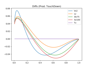
Figure 3: USD/JPY exotics model comparison of 23 Jan 2018, TV of a 9-month One-Touch with a lower barrier on the x-axis, and differences to TV on the y-axis, raw data sourced from Bloomberg, calculations by MathFinance.
The mixture parameter, which is chosen to be 75% in our example, can be calibrated to One-Touch prices, if they are available. We also notice that the vanna-volga approach Vv2, while similar to the other models, is slightly off; therefore, there are market participants using Vv2 for valuation purposes, but a market maker quoting bid and offer prices with a spread of 0.02=2% could potentially be off-market when using Vv2.
This way of illustrating the smile effect for exotics is called the mustache. The reason is that, if you also consider the graph for the One-Touch contracts with an upper barrier in Figure 4, and paste the two graphs next to each other, TouchUp on the left, TouchDown on the right, the combined shape resembles a mustache and is shown in Figure 5. Very touchy.

Figure 4: USD/JPY exotics model comparison of 23 Jan 2018, TV of a 9-month One-Touch with an upper barrier on the x-axis, and differences to TV on the y-axis, raw data sourced from Bloomberg, calculations by MathFinance.
The mustache can be used to visualize how different pricing models capture the volatility smile and can be part of a quantitative model risk analysis. Nowadays, regulators normally require banks to conduct a model risk analysis for all new products to be traded. For front-office it is an important tool to gauge the quality of the in-house model. For this purpose, a number of models need to be implemented, calibrated and contracts priced. For the high-speed, low-tolerance FX derivatives market, gauging and monitoring model risk is crucial for survival.
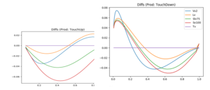
Figure 5: USD/JPY OneTouch Mustache of 23 Jan 2018, TV of a 9-month One-Touch on the x-axes, and differences to TV on the y-axis, raw data sourced from Bloomberg, calculations by MathFinance.
On this year’s MathFinance Conference on 8-9 April we will discuss the recent advance on SLV and other models. As a special feature we have a symposium on crypto currencies, derivatives pricing, risk management, volatility forecasting, followed by a panel discussion with founders of a crypto currency exchange, and expect many delegates with a distinct interest in this field. I am curious myself to find out more and hope to see you in Frankfurt.
Uwe Wystup
Managing Director of MathFinance
MathFinance Conference introduction on https://www.youtube.com/watch?v=3OFcpdC0lWA
Upcoming Events
Thu–Fri, Sept. 12-13, 2019
MATHFINANCE CONFERENCE 2019
Date: April 08 – 09, 2019
Venue: Frankfurt School of Finance & Management, Adickesallee 32-34, 60322 Frankfurt am Main
MathFinance Conference has been successfully running since 2000 and has become one of the top quant events of the year. The conference is specifically designed for practitioners in the areas of trading, quantitative and derivatives research, risk and asset management, insurance, as well as academics.
As always, we expect around 100 delegates both from the academia and the industry. This ensures a unique networking opportunity which should not be missed. A blend of world renowned speakers ensure that a variety of topics and issues of immediate importance are covered.
Please click here for registration (single / group):
Academics pay 525 EUR (+VAT) at all times. We kindly ask for proof of your affiliation.
Group prices (3 or more from the same institution) are at EUR 735 (+VAT) pp.
Single tickets from February 22, 2019 is EUR 1.050 (+VAT).
Details of the conference can be found here.
MathFinance Conference introduction on https://www.youtube.com/watch?v=3OFcpdC0lWA